Understanding AMM Liquidity Through Greeks

Liquidity provision in automated market makers (AMMs) seems deceptively simple: deposit assets, collect fees, earn yield. While this is operationally correct, it hides what an LP position actually is. An LP position is not a single asset or a fixed basket of assets, it is a dynamically rebalanced portfolio. Its composition changes mechanically as trades occur and prices move. Consequently, the value of an LP position is a non-trivial function of market price, time, and volatility. Portfolios with similar structure are well understood in traditional finance. They exhibit: directional exposure, convexity, time-dependent cash flows, and sensitivity to volatility. In the language of finance, those are called Greeks, and they encapsulate how their value responds to changes in the market. Therefore, this provides a natural framework to describe AMMs: Liquidity provision in AMMs is simply an on-chain implementation of a complex portfolio, subject to the same risk decomposition that applies throughout traditional finance. ### Disclaimer: Toxic Flow All of the analysis below implicitly assumes that price motion is largely random, so that volatility provides a meaningful summary of risk. This assumption breaks down when traders interact with the pool primarily when they possess informational or timing advantages. Another important disclaimer is that fees and blocktimes (both average duration and statistics) modify the statistical properties of LVR itself which has been discussed in the literature and is the subject of a forthcoming blog post. --- ## 1️⃣ General Principle: Any Portfolio Has Greeks Henceforth, we measure value in units of a base numeraire (for example USD, ETH, or any chosen reference asset). All portfolio values below are expressed in this unit to allow for meaningful comparisons. Before touching AMMs or any specific market mechanism, we start from the most general object one can write down: a portfolio value function $V = V(p,t,\sigma)$, where V denotes the current value of the portfolio in the chosen numeraire. This value depends on three fundamental variables: - $p$ — the market price of the traded asset, expressed in the chosen numeraire - $t$ — time, which captures both the passage of time itself and any time-dependent cash flows - $\sigma$ — volatility, a measure of how strongly prices fluctuate over time (volatility can and does also depend on time $t$) Any portfolio whose composition changes with price, accrues cash flows over time, or is exposed to fluctuations must, at least locally, depend on these variables. An AMM LP position naturally satisfies all three conditions: its inventory changes mechanically with price, it earns fees over time, and its risk depends on how volatile the market is. For sufficiently small changes in the underlying variables $(dp, dt, d\sigma)$ the portfolio value changes from $V(p,t,\sigma) \to V(p+dp,t+dt,\sigma+d\sigma)$ and its change can be approximated by a Taylor expansion. To leading orders, this gives: $dV \approx \Delta\,dp + \tfrac12\Gamma(dp)^2 + \Theta\,dt + \nu\,d\sigma,$ where each coefficient captures a specific sensitivity of the portfolio value: $\Delta := \frac{\partial V}{\partial p}, \quad \Gamma := \frac{\partial^2 V}{\partial p^2}, \quad \Theta := \frac{\partial V}{\partial t}, \quad \nu := \frac{\partial V}{\partial \sigma}.$ The symbols $\Delta, \Gamma, \Theta, \rm{and}\, \nu$ are a subset of what is traditionally called the Greeks. Mathematically speaking, they are the partial derivatives of the value function V, evaluated at the current state of the market. In other words, the Greeks quantify how the portfolio reacts locally to small changes in price, the passage of time, and market volatility. --- ## 2️⃣ Benchmarks for Performance Risk or performance are meaningless without a benchmark. A portfolio does not “gain” or “lose” value in isolation; it outperforms or underperforms a benchmark. Without stating that reference point explicitly, discussions of risk quickly become ambiguous or misleading. This issue appears repeatedly in the context of liquidity provision. Two quantities are commonly discussed: impermanent loss (IL) and loss-versus-rebalancing (LVR). Both are real, both describe underperformance, and both are attributed to similar underlying mechanics. As a result, they are frequently conflated. In reality, IL and LVR are not competing explanations of the same phenomenon. They arise from different choices of benchmark. IL measures LP performance relative to a static HODL portfolio, while LVR measures performance relative to a continuously rebalanced, delta-neutral portfolio. Once the benchmark is fixed, the relevant source of underperformance becomes unambiguous. To make that distinction precise, we treat benchmarks as explicit reference frames and measure value relative to them. Then IL and LVR correspond to different Greek components of the same portfolio, but different reference frames. We define $P$ as the difference between the actual portfolio value $V$ and the benchmark portfolio value $B$: $P := V - B.$ Then the Greeks of $P$ are: $\Delta_P = \Delta_V - \Delta_B,\quad$ $\Gamma_P = \Gamma_V - \Gamma_B,\quad$ $\Theta_P = \Theta_V - \Theta_B,\quad$ $\nu_P = \nu_V - \nu_B.$ ## 3️⃣ LP Value vs HODL An LP enters (at ’mint’) the pool with an initial inventory $(x_0,y_0)$ at an entry price $p_0$ according to the rules specified by the AMM invariant. We assume that $x$ is the volatile asset and $y$ is the numeraire and the price is measured in units numeraire/volatile asset. For a generic AMM, the LP does not actively trade or rebalance. Instead, the inventory evolves deterministically according to the rules of the AMM as swaps occur: At any price p, the LP holds an updated inventory $(x(p),y(p))$. In addition to inventory changes, LPs earn fees over time. At a time $t$ we can write the total LP value as $V_{\rm LP}(p,t,\sigma) = p \;x(p) + y(p) + \int_0^t f(\tau,\sigma(\tau))\,d\tau$ where the first two terms represent the current value of the LP’s inventory expressed in the numeraire, and the final term represents cumulative fee income up to time t. In this case, $f(t,\sigma(t))$ denotes the instantaneous fee income rate (we allow for volatility to depend on time, in the statistical treatment it is assumed instantaneous). The variables make two points explicit: 1. Fee income is time-dependent, it accrues continuously as trading occurs. 2. Fee income depends on market conditions, in particular on volatility $\sigma$, either implicitly (via volume) or explicitly (via dynamic fee rules) (there are also feedback loops that we disregard). The relevant Greeks of the LP position are: $\Theta_{\rm LP} = \frac{\partial V_{\rm LP}}{\partial t} = f(t,\sigma)$ and $\nu_{\rm LP}=\frac{\partial V_{\rm LP}}{\partial \sigma}=\int_0^t \frac{\partial f(\tau,\sigma)}{\partial \sigma}\, d\tau$. To assess LP performance, we must compare this evolving portfolio to a benchmark. The most natural benchmark is a HODL portfolio that simply keeps the initial inventory $(x_0,y_0)$ unchanged. Its value at price $p$ is $V_{\rm HODL}(p) = p\;x_0 + y_0$. We define LP performance relative to this benchmark as $P^{\rm{HODL}} := V_{\rm LP} - V_{\rm HODL}.$ Differentiating $P^{\rm{HODL}}$ with respect to $(p,t,\sigma)$ gives the local performance decomposition $dP^{\rm{HODL}} \;\approx\; (\Delta_{\rm LP}-\Delta_{\rm HODL})\,dp \;+\; \tfrac12\Gamma_{\rm LP}dp^2 \;+\; \Theta_{\rm LP}\,dt \;+\; \nu_{\rm LP}\,d\sigma$ . This equation summarizes all sources of LP gains and losses relative to HODL: directional effects, curvature effects, fee income, and volatility sensitivity. --- ## 4️⃣ What is Impermanent Loss? The performance measure constructed above is adequate to introduce the concept of IL. Both LP and HODL start from the same inventory: $x(p_0)=x_0,\quad y(p_0)=y_0,$ and their first-order exposure to price must match: $\Delta_{\rm LP}(p_0) = \Delta_{\rm HODL}(p_0).$ Thus locally at mint (t=0), we have $V_{\rm{LP}} = V_{\rm{HODL}}$ and deviations only start from second order. IL arises because this equality holds only at a single point. As price moves away from $p_0$, the LP's delta evolves differently than HODL's, creating a cumulative divergence in value (for a visualization check Figure 1, left-hand-side). We define the delta-difference: $\Delta_P^{\rm{HODL}}(p) := \Delta_{\rm LP}(p) - \Delta_{\rm HODL}(p)$ which leads to a general definition of IL: $\boxed{ \text{IL}(p_1) = V_{\rm LP}(p_1) - V_{\rm HODL}(p_1) =\int_{p_0}^{p_1} \frac{d}{dp}\left( V_{\rm LP}(p) - V_{\rm HODL}(p)\right)dp =\int_{p_0}^{p_1} \Delta_P^{\rm{HODL}}(p)\, dp. }$ A straightforward interpretation follows: IL is the cumulative effect of having a different delta than HODL as price moves and it only depends on start and end point. To second-order can this be approximated as curvature: $\Delta_P^{\rm{HODL}}(p) = O(p-p_0) \;\Longrightarrow\; \text{IL}(p_1) \approx \frac12\Gamma_{P^{\rm HODL}}(p_0) (p_1 - p_0)^2=\frac12(\Gamma_{\rm LP}(p_0)-\Gamma_{\rm HODL}(p_0)) (p_1 - p_0)^2=\frac12\Gamma_{\rm LP}(p_0) (p_1 - p_0)^2.$ leading to statements like ‘IL is a curvature or $\Gamma$ effect’. (Note that $\Gamma_{\rm LP}$ is negative!) However, as shown above, curvature is not the essence of IL, it is simply the local Taylor approximation of the Δ-difference integral. ### A concrete example: A CPMM For constant-product AMMs (reserve invariant ($xy=k$)), we have: $x(p) = \sqrt{\frac{k}{p}},\quad y(p)=\sqrt{kp},$ $V_{\rm LP}(p) = p\; x(p)+y(p)= 2\sqrt{kp},$ where $p=y/x$. The HODL reference value is given by: $V_{\rm HODL}(p) = p\; x_0 + y_0.$ These curves touch at $p_0$ but $V_{\rm LP}(p)$ is strictly concave, $V_{\rm HODL}(p)$ is linear in ($p$). Therefore: $V_{\rm LP}(p) \le V_{\rm HODL}(p)\quad\text{for all }p\ne p_0.$ For a visualization check again the left-hand-side of Figure 1.  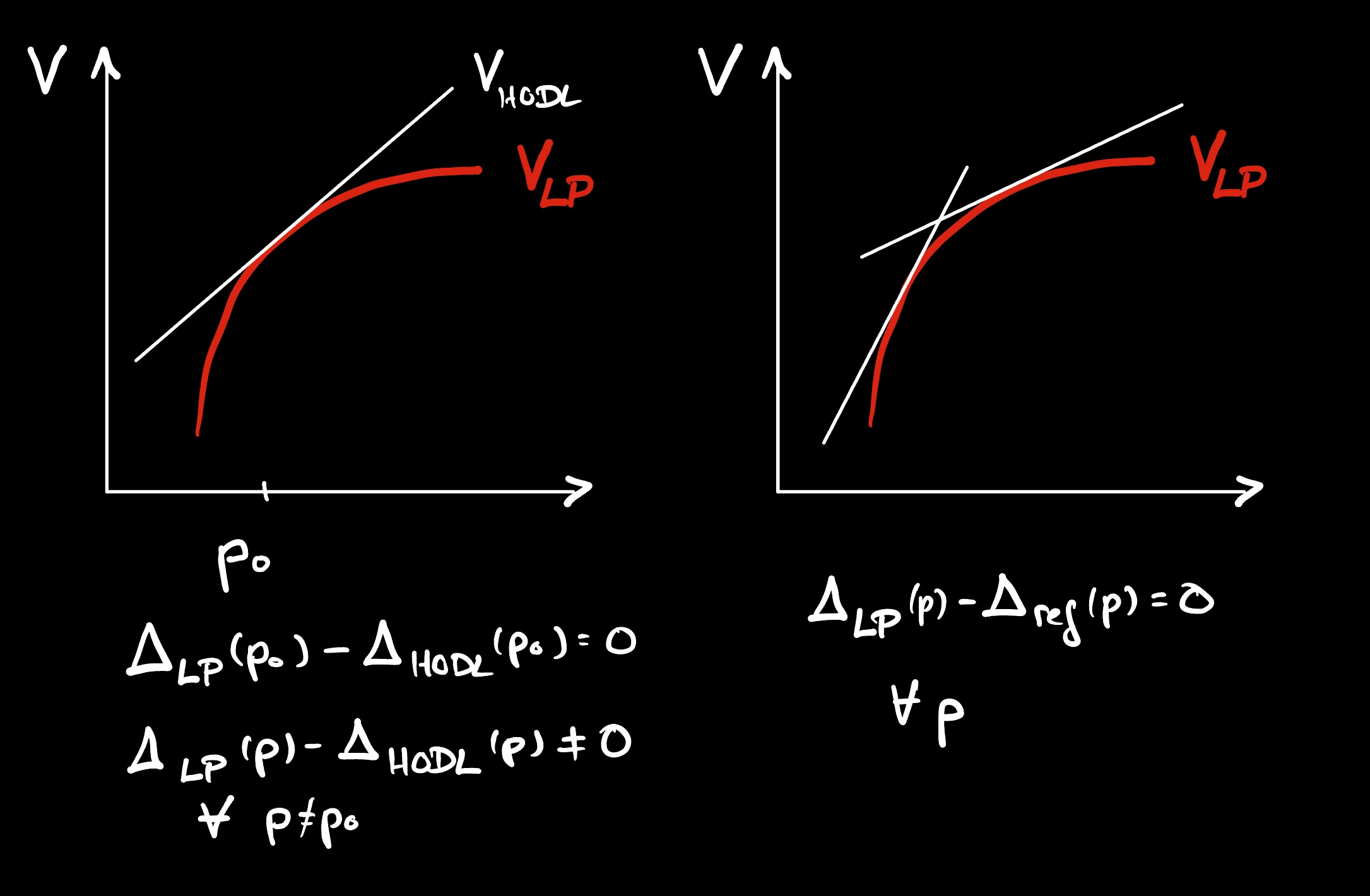Figure 1: Left-hand-side: A generic LP portfolio underperforms relative to a HODL portfolio and they are identical at mint at price $p_0$ (or whenever price returns there). At this point only, the performance P benchmark is delta-neutral, at all other prices it is not delta-neutral. Right-hand-side: If a LP portfolio is compared to a rebalancing portfolio at each price, $V_{\rm{LP}}$ is always tangential to the rebalancing portfolio making the benchmark delta neutral (delta-flat) and strictly concave. --- ## 5️⃣ Loss-versus-rebalancing: The Γ-Bleed of a $\Delta$ neutral portfolio We switch from a HODL benchmark to a $\Delta$-neutral benchmark, and introduce loss-versus-rebalancing (LVR). Instead of comparing the LP to a static portfolio, we compare it to a continuously rebalanced benchmark. After each infinitesimal price change dp, the benchmark is reset so that its delta matches the LP’s delta at the current price (see Figure 1, right-hand-side for an illustration). Equivalently: the benchmark tracks the local slope of the LP value function at all times. This construction removes directional exposure by design. The resulting performance measure, which we denote by $P^{\rm flat}$, satisfies $\Delta_{P}^{\rm flat}= 0$ at every instant. What remains is the pure effect of curvature and higher-order terms. Under this benchmark, the differential performance reduces to $dP^{\rm flat} \approx \tfrac12\Gamma_{\rm LP}(dp)^2+\Theta_{\rm LP}dt+\nu_{\rm LP}d\sigma$. At first glance, this looks like a small correction: the leading linear term in $dp$ has vanished (by choice of the rebalancing reference point), and only quadratic and time-dependent contributions remain. Important note (why LVR is “per trade”) - Strictly speaking, LVR is most naturally defined swap-by-swap which is one of the reasons it is sometimes used to describe informed trades. - The $\Delta$-matched benchmark is constructed right before a swap, so the reference point effectively resets after each execution. - Each swap therefore has a well-defined execution wedge: the gap between paying an average curve price and leaving the pool at a new marginal price (or oracle price). - Over a time window, “total LVR” is simply the sum of these per-swap wedges. ### Statistical properties of LVR In diffusion-style models, this cumulative sum has an expected drift that we derive below. We assume that the price follows a stochastic process of the form $dp = \mu dt + \sigma dW,$ with $dW$ being a Wiener increment, $\sigma$ the volatility, and $\mu$ being the drift (assumed zero for now). In the framework of Itó calculus, the expected quadratic variation of the price satisfies $\langle (dp)^2\rangle \approx \sigma^2\,dt$. Crucially, this term is of the same order in $dt$ as the fee income term $\Theta_{\rm LP}dt$ discussed later. As a result, even though second order in $dp^2$, the curvature contribution does not vanish in the continuous-time limit. Instead, it accumulates over time whenever volatility is non-zero. This leads to the definition of LVR as the positive cost to LPs: $\boxed{\frac{d{\rm LVR}}{dt} \approx -\tfrac12\Gamma_{\rm LP}\sigma^2,}$ where importantly $\Gamma_{\rm LP}<0$. Thus, LVR measures the systematic underperformance of an LP position relative to a continuously rebalanced, delta-neutral benchmark, under statistical price evolution. ## Analogy with options In general, an LP position is ‘short $\Gamma$’. If delta-hedged by continuous rebalancing, it behaves, at a local level, like a short straddle. - it collects premium over time ($\Theta$), - it is short $\Gamma$ and loses when prices move, - and it must earn enough premium to offset the volatility bleed $-\Gamma\sigma^2$ in order to break even. The key difference is structural: AMMs cannot choose a strike, adjust maturity, or exit the position at will. Their exposure is **continuous, automatic, and involuntary**, making LVR a built-in friction of the mechanism rather than a discretionary trading choice. ## 🔹 Trend Exposure vs. Pricing Wedge IL and LVR aren’t competing explanations. They are the same LP payoff viewed against different benchmarks. - IL (vs HODL) = endpoint / trend exposure. It depends only on the start and end price: ${\rm IL}(p_1)=V_{\rm LP}(p_1)-V_{\rm HODL}(p_1) =\int_{p_0}^{p_1}\big(\Delta_{\rm LP}(p)-\Delta_{\rm HODL}(p)\big)\,dp.$ IL is path-independent. No execution rule can remove it, it is about managing inventory. Mitigating IL requires external directional hedging including rebalacing. - LVR (vs $\Delta$-matched rebalancing) = pricing wedge along the path. The $\Delta$-matched benchmark enforces $\Delta_{P^{\rm flat}}\equiv 0$, so performance is driven by curvature sampled by quadratic variation: $\mathbb{E}[dP^{\rm flat}] \approx \tfrac12\Gamma_{\rm LP}\sigma^2\,dt, \qquad {\rm LVR}(0,T)\approx -\int_0^T \tfrac12\Gamma_{\rm LP}\sigma^2\,dt,$ with $T$ being the time horizon of observation. In AMMs this is naturally interpreted swap-by-swap as an execution wedge between an average curve price and the new marginal/oracle price, often captured by arbitrageurs. Since it is an execution-wedge object, it is a legitimate target for execution-rule changes (batching, marginal/tick-boundary pricing, etc.) and/or dynamic fees. In short: IL = where you end up. LVR = what happens while getting there. --- ## 6️⃣ LP Fees as Θ: The Time-Drift of LP Value Since the LP value can be written as $V_{\rm LP} = \text{holdings} + \int f\,dt, \quad \Theta_{\rm LP} = f,$ the Greek $\Theta$ has a very direct interpretation in the AMM context. It measures how much value an LP earns from fees simply because time passes (there are a number of hidden assumptions in this specified below). Equivalently, $\Theta_{\rm LP}$ is the instantaneous fee income rate. It captures the flow of revenue generated by trading activity in the pool. Importantly, this contribution is not guaranteed: if there is no volume, fee income vanishes, regardless of how long the position is held. All profitability statements involving $\Theta$ therefore implicitly assume the presence of sustained trading activity. Once this is made explicit, break-even conditions follow naturally by comparing fee income to the loss mechanisms identified earlier. | **Objective** | **Mathematical condition** | | --- | --- | | break even vs $\Delta$-neutral benchmark | $\Theta_{\rm LP} \ge -\tfrac12\Gamma_{\rm LP}\sigma^2$ | | outperform HODL benchmark | $\int_0^T dt \Theta_{\rm LP}(t) \ge -{\rm IL}$ | where $T$ is the time horizon of observation. The first condition states that, in a volatile market, fee income must at least compensate the curvature-driven volatility bleed described by LVR. The second states that, relative to simply holding the assets, fee income must offset the directional underperformance encoded in IL. Most LP’s underperformance can be traced back to violations of these conditions: fees are simply too small relative to the risks taken. Without sufficient $\Theta$, even a well-designed AMM will systematically underperform its natural benchmarks. Unlike IL which depends only on endpoints, LVR accumulates along the path. This path-dependence creates qualitatively different statistical properties, as shown in Appendix A. --- ## 7️⃣ Vega $\nu$: Dynamic Fees So far, we noted that LPs are exposed to both directional risk ($\Delta$) and volatility-driven curvature risk ($\Gamma$). It is therefore natural to ask whether LP compensation responds to changes in market volatility. In many major AMMs today, the instantaneous fee income rate f is fixed by protocol parameters and does not depend explicitly on volatility. In that case, $\frac{\partial f}{\partial \sigma} = 0 \quad\Longrightarrow\quad \nu_{\rm LP} = 0$. The economic implication is straightforward: LPs bear more risk when markets become volatile, but are not paid more for doing so. As volatility increases, LVR grows through the $\Gamma\sigma^2$ term, while fee income remains unchanged (obviously, volume will respond in these cases so there is an indirect effect). In Greek language, LPs are short gamma but have no vega. Dynamic-fee mechanisms address this mismatch by allowing fee income to respond to market conditions in a direct manner. In such systems, the instantaneous fee rate is itself a function of volatility, $\Theta_{\rm LP} = \Theta_{\rm LP}(\sigma), \qquad \nu_{\rm LP} = \frac{\partial \Theta_{\rm LP}}{\partial \sigma} > 0.$ This introduces an explicit volatility sensitivity of LP returns: when markets become more volatile and LP risk increases, fee income rises accordingly. From a portfolio perspective, dynamic fees do not eliminate volatility risk, but they compensate it. Implementing such mechanisms in practice requires a way to estimate or proxy volatility. Possible approaches include: - using realized volatility computed from recent on-chain price returns, - incorporating implied volatility from oracle or derivative markets, - or reacting to local shocks, for example by increasing fees on unusually large or sudden trades. In this framework, $\nu$ measures whether compensation increases with volatility. --- ## 8️⃣ Summary Locally in price, time, and volatility, the value of an LP position evolves according to $dV_{\rm LP} \;\approx\; \Delta\,dp + \tfrac12\Gamma_{\rm LP}(dp)^2 + \Theta\,dt + \nu\,d\sigma.$ Different benchmarks ‘project’ this same object onto different components: - vs HODL: performance is dominated by the $\Delta$ mismatch** → IL (endpoint). - vs $\Delta$-matched rebalancing: the $\Delta$ term cancels by construction, leaving curvature sampled by quadratic variation → LVR (path). - $\Theta$: fee drift (income per unit time). - $\nu$: whether compensation increases with volatility (dynamic fees). | **Effect** | **Greek** | **Interprets as** | | --- | --- | --- | | Endpoint exposure | $\Delta$ | IL vs HODL | | Path / volatility bleed | $\Gamma$ | LVR vs Δ-neutral benchmark | | Fee income | $\Theta$ | fee drift | | Volatility-priced fees | $\nu$ | dynamic fee response | Two paths with the same start and end price can have identical IL but very different LVR, see Appendix A for an extreme example. ### Different questions imply different benchmarks - LP deciding to withdraw: compare to HODL → “Did I beat holding?” (IL is the relevant gap.) - Protocol fee design: compare to $\Delta$-neutral expectation → “Do fees cover volatility bleed?” (Need $\Theta \gtrsim |\tfrac12\Gamma\sigma^2|$.) - Professional market maker: compare passive LP to active hedging → both IL ($\Delta$ exposure) and LVR (automation/$\Gamma$-bleed) matter. ### 🧭 Hedging Insight: What Fees Can and Cannot Offset Once the Greek structure is explicit, it becomes possible to ask which risks can be mitigated internally through AMM design, and which require external instruments. - LVR, which arises from volatility-driven curvature effects, can be mitigated, at least in principle, by dynamic fees. Introducing a positive vega ensures that fee income increases when volatility rises: $\frac{\partial \Theta_{\rm LP}}{\partial \sigma} > 0.$ This does not remove volatility risk, but it compensates LPs for bearing it. - IL, by contrast, $\text{IL}(p_1) = \int_{p_0}^{p_1} \big(\Delta_{\rm LP}(p)-\Delta_{\rm HODL}(p)\big)\,dp,$ is fundamentally a directional effect. It depends only on the terminal price and reflects the fact that the LP’s delta profile differs from that of a static HODL portfolio. No fee mechanism, fixed or dynamic, can hedge this type of loss. Hedging IL therefore requires directional tools, such as offsetting spot exposure, perpetual or futures positions, or options that insure against large endpoint deviations. Put succinctly: Dynamic fees or pricing in general hedge $\Gamma$-risk Directional instruments hedge $\Delta$-risk A complete and sustainable LP ecosystem requires both. They address different dimensions of risk and are complementary rather than substitutable. ## 🏁 Closing The key challenge of liquidity provision is inventory management under uncertainty, and by pricing that uncertainty using the same tools that have governed market making in traditional finance for decades: the Greeks. An LP position is not passive yield. It is a portfolio with exposure to price levels, price paths, time, and volatility. Once that is acknowledged, the relevant questions become unavoidable: - $\Delta$ asks: Where will the price end? - $\Gamma$ asks: How violently will the path wander before it gets there? - $\Theta$ asks: Does the mere passage of time generate sufficient compensation? - $\nu$ asks: Is volatility itself actually being priced? Most failures in LP economics stem from ignoring one or more of these dimensions. In particular, an AMM that offers $\Theta$ but effectively sets $\nu \approx 0$ is equivalent to a market-maker forced to quote the same spread during a quiet Sunday market and a macro announcement shock. Risk changes, but compensation does not. The Greeks framework makes this mismatch explicit. It clarifies which losses are structural, which are benchmark-dependent, and which can be mitigated through design. More importantly, it provides a common language in which AMMs, dynamic fees, and derivative overlays can be discussed without confusion. Addressing toxic flow requires additional microstructural mechanisms, such as flow filtering, oracle smoothing, batch auctions, or other designs that distinguish benign from informed trading. One such mechanism will be discussed in a forthcoming post. --- **Some References** 1. Bardoscia, N., & Nodari, A. (2023). *Liquidity Providers Greeks and Impermanent Gain*. arXiv:2302.11942. Explicit computation of Δ, Γ, Θ, ν for AMM positions and hedging proposals. 2. Milionis, J., Moallemi, C. C., Roughgarden, T., & Zhang, A. L. (2022). *LVR: Quantifying the Cost of Providing Liquidity to Automated Market Makers*. a16z crypto Research. Foundational introduction of LVR as adverse-selection cost and distinction from IL. 3. Baggiani, L., Herdegen, J., & Macrina, A. (2025). *Optimal Dynamic Fees in Automated Market Makers*. arXiv:2506.02869. Derivation of volatility- and inventory-responsive dynamic fees to offset LVR/IL. 4. Lebedeva, A., & Umnov, A. (2025). *Dynamic Fee for Reducing Impermanent Loss in Decentralized Exchanges*. IEEE Xplore. Proposal and analysis of dynamic fee mechanisms to address IL/LVR. 5. Kim, Y. (2021, updated). *Liquidity Provision by Automated Market Makers*. SSRN:3674178. Game-theoretic treatment of adverse selection and liquidity provision incentives. 6. Mamageishvili, A., & Felten, E. (2024). *The Cost of Permissionless Liquidity Provision in Automated Market Makers*. arXiv:2402.18256. Analysis of excess liquidity and adverse selection costs due to proportional fees. ## **📎 Appendix A — Impermanent Loss and Loss-Versus-Rebalancing Revisited** This appendix clarifies the precise relationship between **Impermanent Loss (IL)** and **Loss-Versus-Rebalancing (LVR)**. Both quantities describe underperformance of an AMM LP position, and both originate from the same underlying curvature of the AMM value function. Nevertheless, they correspond to **different benchmarks** and capture **fundamentally different aspects of risk**. The purpose of this appendix is to make this distinction introduced above in a theoretical framework more explicit and transparent and to reconcile several statements that are often treated as contradictory. --- ### A.1 Benchmark Choice Is the Only Difference Throughout the main article, performance is defined relative to a benchmark B, $P := V - B.$ IL and LVR arise from the same LP portfolio, but with different benchmark choices: - Impermanent Loss (IL) benchmarks against a static HODL portfolio with fixed inventory $(x_0,y_0)$. - Loss-Versus-Rebalancing (LVR) benchmarks against a continuously rebalanced ($\Delta$-matched) portfolio. Once this distinction is made, the apparent tension between IL and LVR disappears. --- ### A.2 Impermanent Loss: Endpoint Performance vs. HODL Impermanent loss measures LP performance relative to HODL at a **single final price** p_1. By definition, $\text{IL}(p_1) = V_{\rm LP}(p_1)-V_{\rm HODL}(p_1).$ Using the fundamental relation $\frac{d}{dp}\big(V_{\rm LP}(p)-V_{\rm HODL}(p)\big) = \Delta_{\rm LP}(p)-\Delta_{\rm HODL}(p),$ IL admits the exact representation $\boxed{ \text{IL}(p_1) = \int_{p_0}^{p_1} \big(\Delta_{\rm LP}(p)-\Delta_{\rm HODL}(p)\big)\,dp. }$ This expression makes the nature of IL precise: - IL is the integral of the delta mismatch between LP and HODL. - IL depends only on the endpoints $p_0$ and $p_1$. - IL is path-independent. For constant-product AMMs, this integral evaluates to the familiar closed-form expression depending only on the price ratio $p_1/p_0$. --- ### A.3 Loss-Versus-Rebalancing: Path Performance vs. $\Delta$-Neutral Benchmark Loss-versus-rebalancing answers a different question: how much worse does the LP perform relative to a portfolio that is continuously rebalanced to match the LP’s instantaneous delta? By construction, this benchmark removes first-order price exposure, $\Delta_{P^{\rm flat}} = 0$, so that performance evolves as $dP^{\rm flat} \;\approx\; \tfrac12\Gamma_{\rm LP}(dp)^2.$ Under stochastic price dynamics $dp = \mu\,dt + \sigma\,dW,$ quadratic variation implies $(dp)^2 \sim \sigma^2 dt,$ leading to the standard approximation $\boxed{ \text{LVR} \;\approx\; \tfrac12\Gamma_{\rm LP}\sigma^2. }$ Thus: - LVR is path-dependent - LVR accumulates with realized volatility - LVR persists even if price returns to $p_0$ --- ### A.4 Same Curvature, Different Projections Both IL and LVR originate from the same curvature of the LP value function. The difference lies in *how that curvature is sampled*. - IL integrates the delta difference along price: $\text{IL} = \int_{p_0}^{p(T)} \Delta_P(p)\,dp.$ - LVR integrates the quadratic variation along the path: $\text{LVR} \sim \int \Gamma_{\rm LP}(dp)^2=\int_0^T dt \frac{1}{2}\Gamma_{\rm{LP}}\sigma^2(t).$ where T is the observation duration. The first is endpoint geometry. The second is path accumulation. Consequently, IL and LVR can coincide in expectation under random price motion, yet differ dramatically for realized paths. This becomes particularly apparent if one studies the statistics of the quantities under geometric Brownian motion. To show this we performed a series of Monte Carlo runs that simulated 2000 geometric Brownian price paths with a length of 5000 time steps (initial price $p_{\rm{init}}=100$ and $\sigma_0=0.01$). The results are shown in Figure 2. IL exhibits tails driven by rare large endpoint deviations, while LVR concentrates tightly around its mean due to incremental accumulation. Interestingly, both show the same mean value, though.   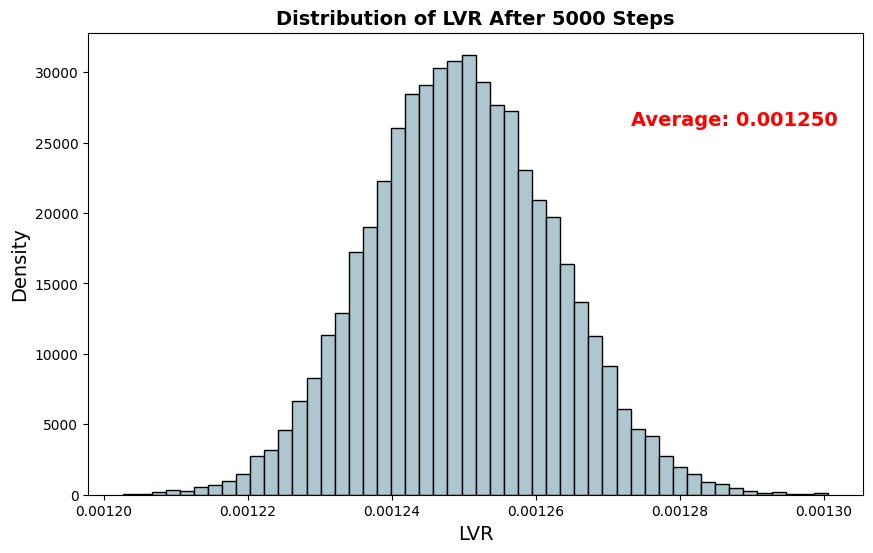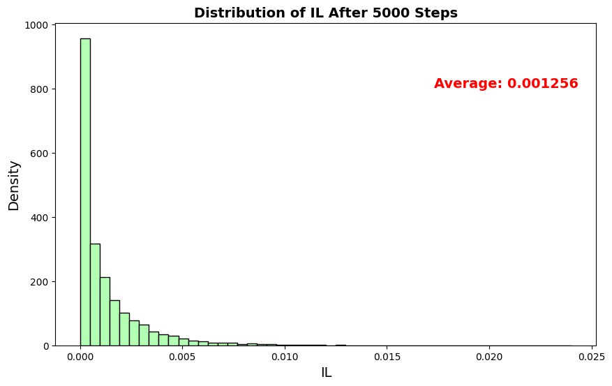Figure 2: The distribution of LVR and IL over 2000 simulated price paths with a length of 5000 time steps (initial price $p_{\rm{init}}=100$ and $\sigma_0=0.01$) shows this contrast starkly, LVR has a narrow peak, while IL has heavy tails. --- ### A.5 Smooth-Path Limit: Why IL Survives and LVR Vanishes Consider a fixed total price change $\Delta p$ decomposed into N small steps $dp = \Delta p/N$, see Figure 3. Then: $\text{LVR} \sim \sum (dp)^2 = N\left(\frac{\Delta p}{N}\right)^2 = \frac{(\Delta p)^2}{N} \;\xrightarrow[N\to\infty]{}\;0,$ while $\text{IL} \sim (\Delta p)^2,$ independent of N.  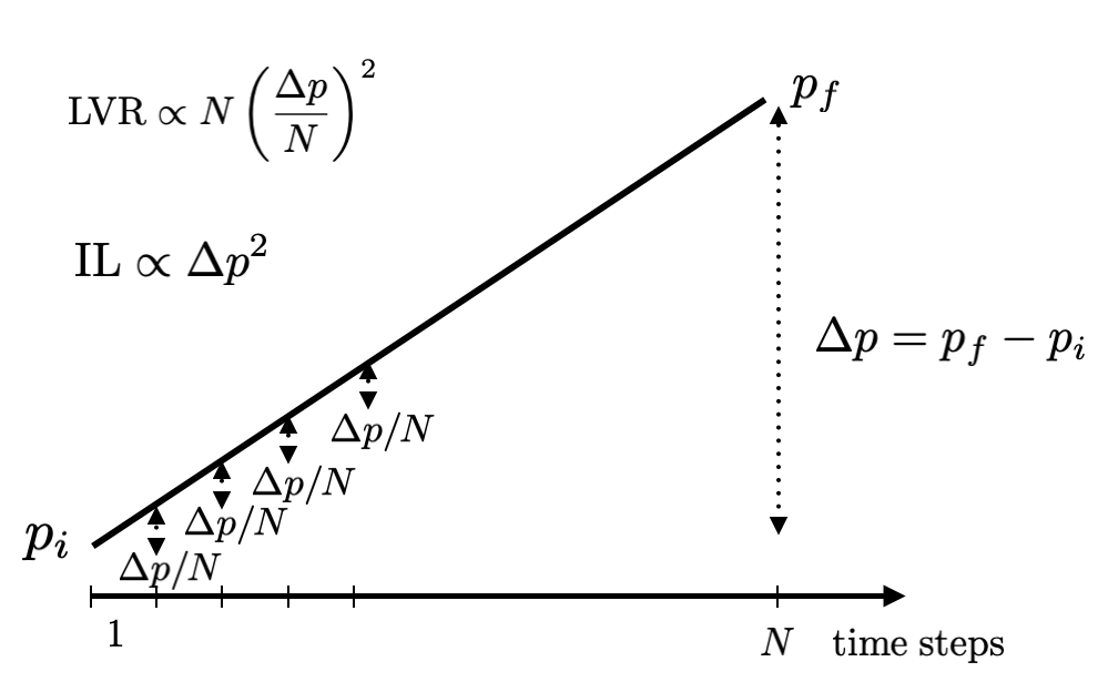Figure 3: Breaking up one step into many small steps effectively eliminates LVR (since it always resets) but does not change IL. This is in line with the interpretation that IL only cares about end point vs. starting point while LVR cares only about the path. This illustrates a fundamental asymmetry: > Infinitely frequent rebalancing eliminates LVR but leaves IL unchanged. > IL is therefore structural, while LVR is a path effect. Note that this discussion is not a discussion of statistical properties of LVR which is presented in an upcoming blog post --- ### A.6 Implications for Arbitrage and Execution This distinction has direct consequences for arbitrage behavior: - Frequent arbitrage reduces LVR, benefiting LPs. - Infrequent arbitrage allows deviations to build, increasing LVR and benefiting arbitrageurs. IL, however, is unaffected by arbitrage timing, it depends only on the terminal price. Thus execution speed influences LVR but not IL. --- ### A.7 Summary - IL measures endpoint underperformance relative to HODL. - LVR measures path-dependent underperformance relative to a $\Delta$-neutral benchmark. - Both arise from curvature, but correspond to different benchmarks. - LVR can be mitigated by execution speed and dynamic fees. - IL persists even in the limit of perfect rebalancing. IL and LVR are not competing notions. They are different benchmark-dependent projections of the same underlying LP payoff structure.